Instructions

• Due date: 11:59pm on Wednesday, November 2nd, 2016

• Handin: through Canvas

• Starter code and data: hw4.zip

• Deliverables:

  • Please prepare your answer sheet using the filename of FirstName_LastName_HW4.pdf.

  • Include all the code you implement in each problem. Remember to set relative paths so that we can run your code out of the box.

  • Compress the code and answer sheet into FirstName_LastName_HW4.zip before uploading it to canvas.

Part 1: SLIC Superpixels (35 points)

Overview

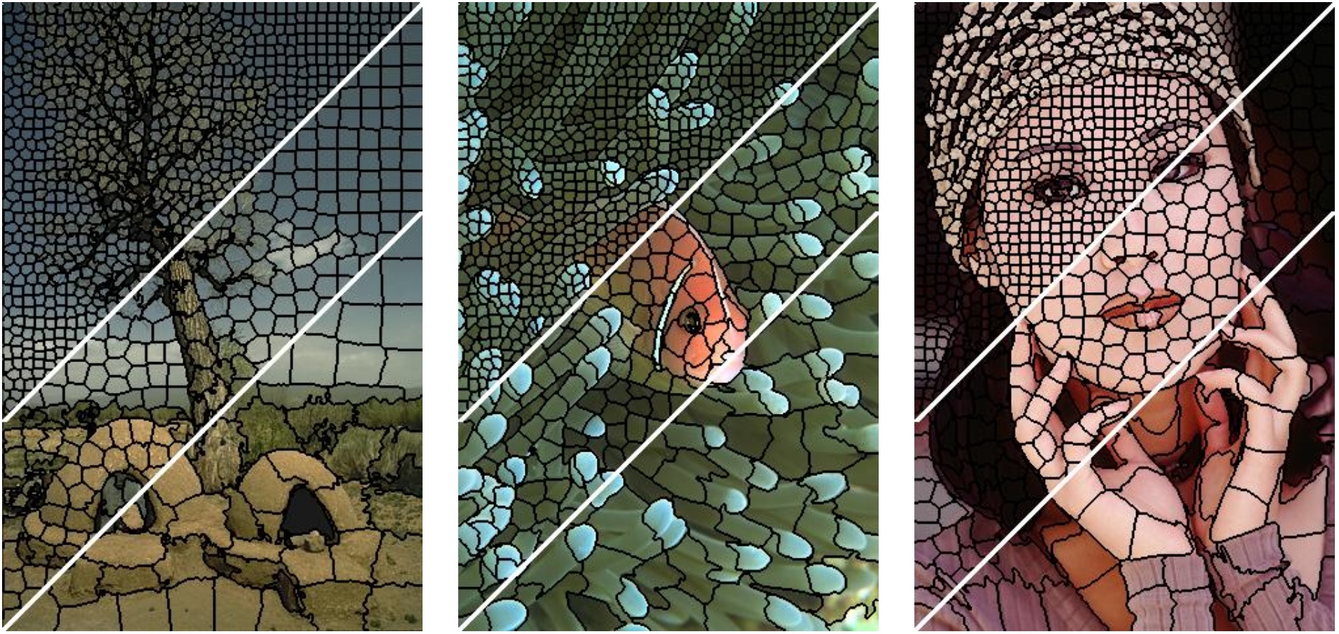
Superpixel algorithms group pixels into perceptually meaningful regions while respecting potential object contours, and thereby can replace the rigid pixel grid structure. Due to the reduced complexity, superpixels are becoming popular for various computer vision applications, e.g., multiclass object segmentation, depth estimation, human pose estimation, and object localization. In this problem, you will implement a simple superpixel algorithm called Simple Linear Iterative Clustering (SLIC) that clusters pixels in the five-dimensional color and pixel coordinate space (e.g., \(r, g, b, x, y\)). The algorithm starts with a collection of K cluster centers initialized at an equally sampled regular grid on the image of N pixels. For each cluster, you define for a localized window 2S x 2S centered at the cluster center, where \(S = \sqrt{N/K}\) is the roughly the space between the seed cluster centers. Then, you check whether the pixel within the 2S x 2S local window should be assigned to the cluster center or not (by comparing the distance in 5D space to the cluster center). Once you loop through all the clusters, you can update the cluster center by averaging over the cluster members. Iterate the pixel-to-cluster assignment process till convergence or maximum iterations reached. For more details, please see SLIC Superpixels Compared to State-of-the-art Superpixel Methods, PAMI 2012.

Write-up

• (5 points) (a) Explain your distance function for measuring the similarity between a pixel and cluster in the 5D space.

• (5 points) (b) Choose one image, try three different weights on the color and spatial feature and show the three segmentation results. Describe what you observe.

• (5 points) (c) Choose one image, show the error map (1) at the initialization and (2) at convergence. Note: error - distance to cluster center in the 5D space.

• (5 points) (d) Choose one image, show three superpixel results with different number of \(K\), e.g., \(64, 256, 1024\) and run time for each \(K\) (use tic, toc)

• (15 points) (e) Run your algorithms on the subset (50 images) of Berkeley Segmentation Dataset (BSD) and report two types metrics (1) boundary recall and (2) under-segmentation error with \(K = 64, 256, 1024\). Also, report averaged run time per image for the BSD

Hint

• Use meshgrid and sub2ind for finding pixel indices for vectorizing your code.

Part 2: EM Algorithm: Dealing with Bad Annotations (35 points)

Dealing with noisy annotations is a common problem in computer vision, especially when using crowd- sourcing tools, like Amazon's Mechanical Turk. For this problem, you've collected photo aesthetic ratings for 150 images. Each image is labeled 5 times by a total of 25 annotators (each annotator provided 30 labels). Each label consists of a continuous score from 0 (unattractive) to 10 (attractive). The problem is that some users do not understand instructions or are trying to get paid without attending to the image. These “bad” annotators assign a label uniformly at random from 0 to 10. Other “good” annotators assign a label to the \(i^{th}\) image with mean \(\mu\) and standard deviation \(\sigma\) (\(\sigma\) is the same for all images). Your goal is to solve for the most likely image scores and to figure out which annotators are trying to cheat you.
In your write-up, use the following notation:

• \(x_{ij} \in [0, 10]\): the score for \(i^{th}\) image from the \(j^{th}\) annotator

• \(m_j \in \{0, 1\}\): whether each \(j^{th}\) annotator is “good” (\(m_j = 1\)) or “bad” (\(m_j = 0\))

• \(P(x_{ij}|m_j = 0) = \frac{1}{10}\): uniform distribution for bad annotators

• \(P(x_{ij}|m_j = 1; \mu_i, \sigma) = \frac{1}{\sqrt{2\pi \sigma^2}} \exp(-\frac{1}{2} \frac{(x_{ij}-\mu_i)^2}{\sigma^2})\): normal distribution for good annotators

• \(P(m_j = 1; \beta ) = \beta\): prior probability for being a good annotator

Derivation of EM Algorithm (20 points)

Derive the EM algorithm to solve for each \(\mu_i\), each \(m_j\), \(\sigma\), and \(\beta\). Show the major steps of the derivation and make it clear how to compute each variable in the update step.

Application to Data (15 points)

You can find the annotation_data.mat " file containing

• annotator_ids(i) provides the ID of the annotator for the \(i^{th}\) annotation entry

• image_ids(i) provides the ID of the image for the \(i^{th}\) annotation entry

• annotation_scores(i) provides the \(i^{th}\) annotated score
  Implement the EM algorithm to solve for all variables. You will need to initialize the probability that each annotator is good { set the initial value to 0.5 for each annotator.
  

Write-up

• (a) Report the indices corresponding to “bad” annotators (\(j\) for which \(m_j\) is most likely \(0\))

• (b) Report the estimated value of \(\sigma\)

• (c) Plot the estimated means \(\mu_i\) of the image scores (e.g., plot(1:150, mean scores(1:150)))

Hint

• For numerical stability, you should use logsumexp.m when computing the likelihood that an annotator is “good”, given the current parameters. The joint probability of each annotators scores and “goodness” will be very small (close to zero by numerical precision). Thus, you should compute the log probabilities and use logsumexp to compute the denominator.

• Another useful functions is normpdf

• In each iteration, show the bar plot of probability of “good” for each annotator and show the plot of the mean score for each image. At the end, you should be very confident which annotators are “good”.

Part 3: Graph-cut Segmentation (30 points)

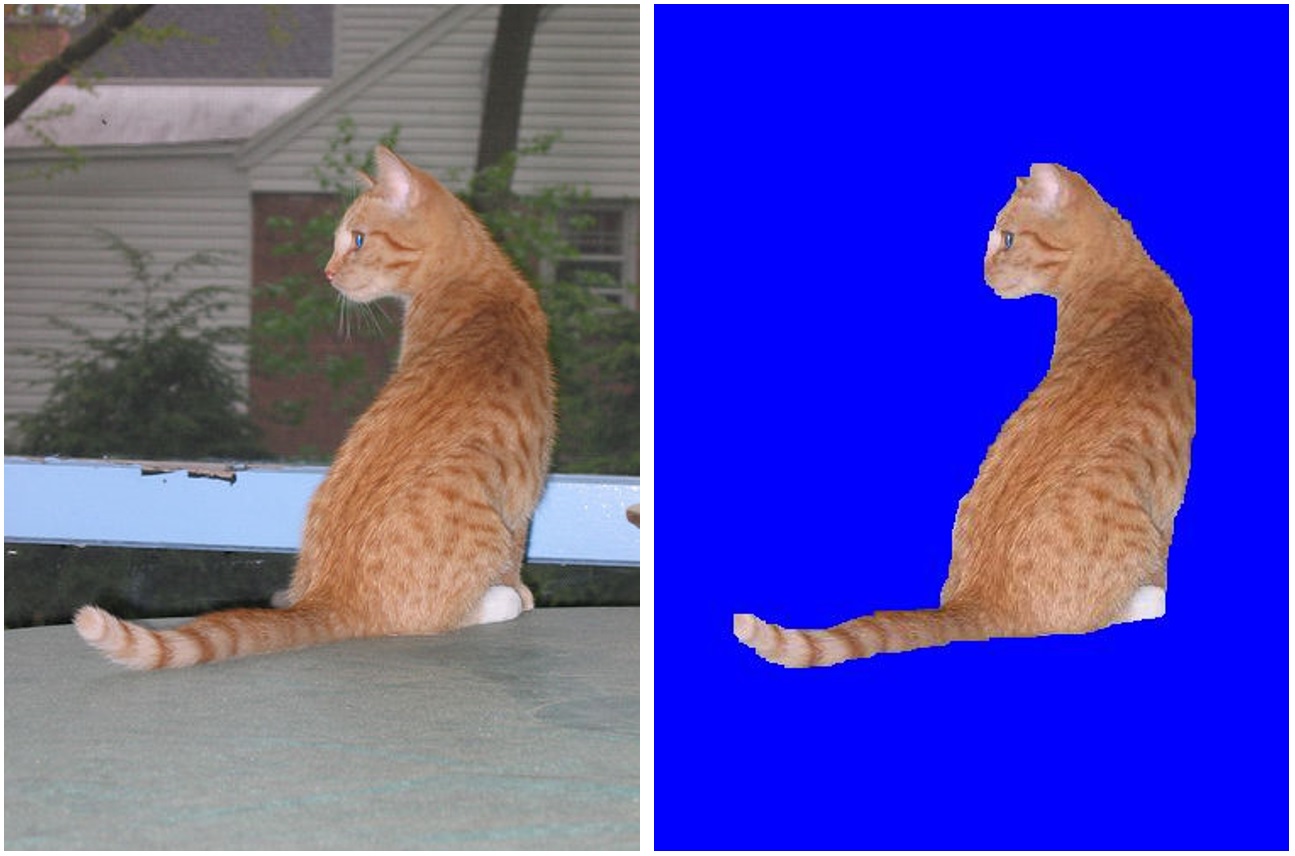Let us apply Graph-cuts for foreground/background segmentation. In the “cat” image, you are given a rough polygon of a foreground cat. Apply Graph-cuts to get a better segmentation. First, you need an energy function. Your energy function should include a unary term, a data- independent smoothing term, and a contrast-sensitive smoothing term. Your unary terms should be \(\log[(\frac{P(\mathrm{pixel}|\mathrm{foreground})}{ P(\mathrm{pixel}|\mathrm{background})}]\). Your pairwise term should include uniform smoothing and the contrast- sensitive term. To construct the unary term, use the provided polygon to obtain an estimate of foreground and background color likelihood. You may choose the likelihood distribution (e.g., color histograms or color mixture of Gaussians.).
Apply graph cut code for segmentation. You must define the graph structure and unary and pairwise terms and use the provided graph cut code or another package of your choice.

Write-up

• (5 points) (a) Explain your foreground and background likelihood function.

• (5 points) (b) Write unary and pairwise term as well as the whole energy function, in math expressions.

• (10 points) (c) Your foreground and background likelihood map. Display \(P(\mathrm{foreground} | \mathrm{pixel})\) as an intensity map (bright = confident foreground).

• (10 points) (d) Final segmentation. Create an image for which the background pixels are blue, and the foreground pixels have the color of the input image.

Hint

• You can use MATLAB GMM functions for estimating the foreground and background distributions.

Extra credit / graduate credit (max possible 30 points extra credit)

SLIC Superpixels

• up to 15 points: Try to improve your result part 1-(e). You may try different color space (e.g., CIELab, HSV) (See Sec 4.5 in the paper), richer image features (e.g., gradients) or any other ideas you come up with. Report the accuracy on boundary recall and under-segmentation error with K = 256. Compare the results with part 1-(e) and explain why you get better results.

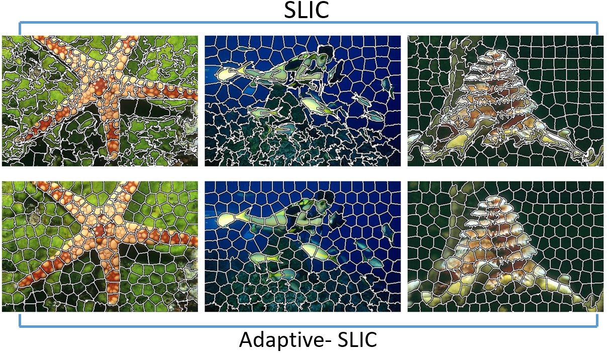
• up to 15 points: Implement Adaptive-SLIC (the parameter-free version of SLIC). See Sec 4.5.E in the paper for more details. Test your Adaptive-SLIC implementation on two images and compare the results with SLIC.

Graph-cut Segmentation

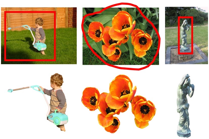
• up to 15 points: Try your Graph-cut implementation on two more segmentation results. Specify the foreground object of interest with a bounding box and use Graph-cut to refine the boundary. Show us (1) the input image, (2) the initial bounding box and (3) the segmentation result.

• up to 10 points: Use your Graph-cut to segment out an object in one image. Then, copy and paste the segmentation onto another image. See here for some ideas.

In your answer sheet, describe the extra points under a separate heading.

Acknowledgements

This homework is adapted from the projects developed by Derek Hoiem (UIUC)