ECE 5554 / ECE 4554: Computer Vision Fall 2016
Instructions
Due date: 11:55pm on Monday, September 19th, 2016
Handin: through https:canvas.vt.edu
Starter code and data: hw1.zip
Deliverables:
Please prepare your answer sheet using the filename of FirstName_LastName_HW1.pdf.
Include all the code you implement in each problem. Remember to set relative paths so that we can run your code out of the box.
Compress the code and answer sheet into FirstName_LastName_HW1.zip before uploading it to canvas.
Part 1: Hybrid image (30 points)
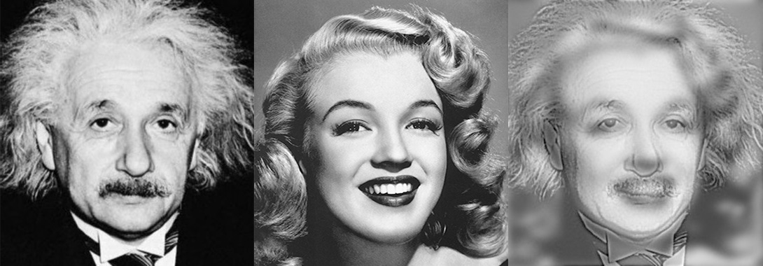 |
Overview
A hybrid image is the sum of a low-pass filtered version of the one image and a high-pass filtered version of a second image. There is a free parameter, which can be tuned for each image pair, which controls how much high frequency to remove from the first image and how much low frequency to leave in the second image. This is called the “cutoff-frequency”. In the paper it is suggested to use two cutoff frequencies (one tuned for each image) and you are free to try that, as well. In the starter code, the cutoff frequency is controlled by changing the standard deviation of the Gausian filter used in constructing the hybrid images.
We provided 7 pairs of aligned images. The alignment is important because it affects the perceptual grouping (read the paper for details). We encourage you to create additional examples (e.g. change of expression, morph between different objects, change over time, etc.).
Write-up
Please provide three hybrid image results. For one of your favorite results, show
(a) the original and filtered images
(b) the hybrid image and hybrid_image_scale (generated using vis_hybrid_image.m provided in the starter code)
(c) log magnitude of the Fourier transform of the two original images, the filtered images, and the hybrid image
Briefly (a few sentences) explain how it works, using your favorite results as illustrations.
Hint
In Matlab, you can compute and display the 2D Fourier transform with with:
imagesc(log(abs(fftshift(fft2(gray_image)))))
Rubric
20 points for a working implementation to create hybrid images from two aligned input images.
10 points for illustration of results: 5 points for input/filtered/hybrid images and 5 points for FFT images.
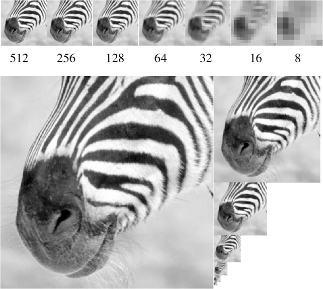
Part 2: Image pyramid (30 points)
Overview
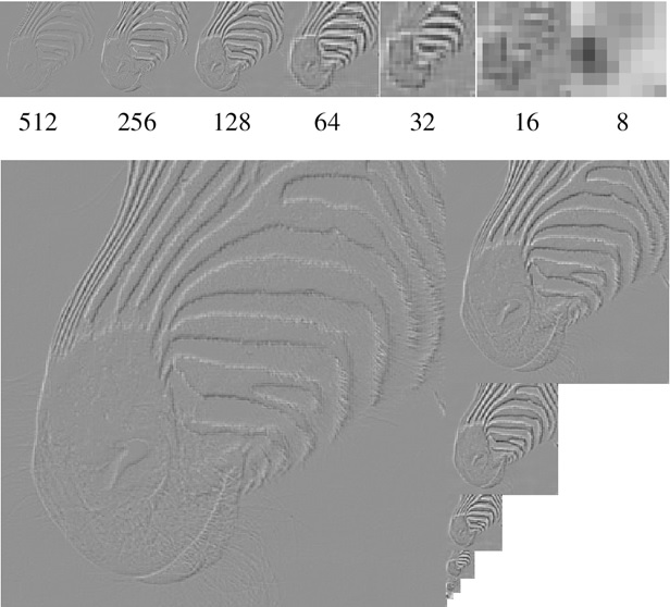
Choose an image that has interesting variety of textures (from Flickr or your own images). The images should be at least 640x480 pixels and converted to grayscale. Write code for a Gaussian and Laplacian pyramid of level N (use for loops). In each level, the resolution should be reduced by a factor of 2. Show the pyramids for your chosen image and include the code in your write-up.
Write-up
(a) Display a Gaussian and Laplacian pyramid of level 5 (using your code). It should be formatted similar to the figure below. You may find tight_subplot.m, included in hw1.zip, to be helpful.
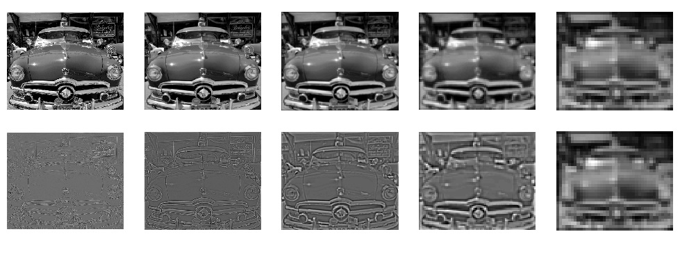 |
(b) Display the FFT amplitudes of your Gaussian/Laplacian pyramids. Appropriate display ranges (using imagesc ) should be chosen so that the changes in frequency in different levels of the pyramid are clearly visible. Explain what the Laplacian and Gaussian pyramids are doing in terms of frequency.
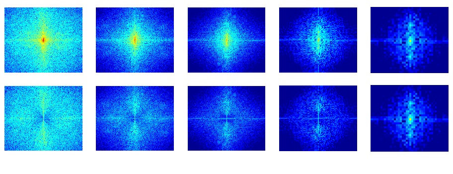 |
Rubric
15 points for a working implementation of Gaussian and Laplacian pyramids.
15 points for displaying the FFT amplitudes of the Gaussian/Laplacian pyramids.
Hint
Useful functions include: imfilter, fft2, cell, figure, subplot, imagesc(im,[minval maxval]), colormap, mat2gray, help/doc
With high-pass filtered images or laplacian pyramid images, many of the values will be negative. To display them, you need to rescale the images to range from 0 to 1 (e.g., with mat2gray ) or use imagesc .
Part 3: Edge detection (40 points)
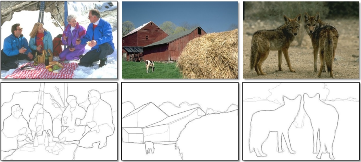 |
Overview
The main steps of edge detection are: (1) assign a score to each pixel; (2) find local maxima along the direction perpendicular to the edge. Sometimes a third step is performed where local evidence is propagated so that long contours are more confident or strong edges boost the confidence of nearby weak edges. Optionally, a thresholding step can then convert from soft boundaries to hard binary boundaries.
I have provided 50 test images with ground truth from BSDS, along with some code for evaluation. Your job is to build a simple gradient-based edge detector, extend it using multiple oriented filters, and then describe other possible improvements. Details of your write-up are towards the end.
(a) Build a simple gradient-based edge detector that includes the following functions
function [mag, theta] = gradientMagnitude(im, sigma)
This function should take an RGB image as input, smooth the image with Gaussian std=sigma, compute the x and y gradient values of the smoothed image, and output image maps of the gradient magnitude and orientation at each pixel. You can compute the gradient magnitude of an RGB image by taking the L2-norm of the R, G, and B gradients. The orientation can be computed from the channel corresponding to the largest gradient magnitude. The overall gradient magnitude is the L2-norm of the x and y gradients. mag and theta should be the same size as im.
function bmap = edgeGradient(im)
This function should use gradientMagnitude to compute a soft boundary map and then perform non-maxima suppression. For this assignment, it is acceptable to perform non-maxima suppression by retaining only the magnitudes along the binary edges produce by the Canny edge detector: edge(im, ‘canny’). Alternatively, you could use the provided nonmax.m (be careful about the way orientation is defined if you do). You may obtain better results by writing a non-maxima suppression algorithm that uses your own estimates of the magnitude and orientation. If desired, the boundary scores can be rescaled, e.g., by raising to an exponent: mag2 = mag.^0.7 , which is primarily useful for visualization. Evaluate using evaluateSegmentation.m and record the overall and average F-scores.
(b) Try to improve your results using a set of oriented filters, rather than the simple derivative of Gaussian approach above, including the following functions:
function [mag,theta] = orientedFilterMagnitude(im)
Computes the boundary magnitude and orientation using a set of oriented filters, such as elongated Gaussian derivative filters. Explain your choice of filters. Use at least four orientations. One way to combine filter responses is to compute a boundary score for each filter (simply by filtering with it) and then use the max and argmax over filter responses to compute the magnitude and orientation for each pixel.
function bmap = edgeOrientedFilters(im)
Similar to part (a), this should call orientedFilterMagnitude, perform the non-maxima suppression, and output the final soft edge map.
Evaluation: The provided evaluateSegmentation.m will evaluate your boundary detectors against the ground truth segmentations and summarize the performance. You will need to edit to put in your own directories and edge detection functions. Note that I modified the evaluation function from the original BSDS criteria, so the numbers are not comparable to the BSDS web page. The overall and average F-score for my implementation were (0.57, 0.62) for part (a) and (0.58, 0.63) for part (b). You might do better (or slightly worse).
Write-up
Include your code with your electronic submission. In your write-up, include:
Description of any design choices and parameters
The bank of filters used for part (b) ( imagesc or mat2gray may help with visualization)
Qualitative results: choose two example images; show input images and outputs of each edge detector
Quantitative results: precision-recall plots (see “pr_full.jpg” after running evaluation) and tables showing the overall F-score (the number shown on the plot) and the average F-score (which is outputted as text after running the evaluation script).
Rubric
25 points for the implementation of a simple gradient-based edge detector as described in (a).
15 points for the implementation of improving the edge detector using oriented filters as described in (b).
Hint
Reading these will aid understanding and may help with the assignment.
Extra points (up to 5 points each, max possible 30 points extra credit)
In your answer sheet, describe the extra points under a separate heading.
Hybrid image
Show us at least two more hybrid image results that are not included in the homework material, including one that doesn't work so well (failure example). Briefly explain how you got the good results (e.g., chosen cut-off frequencies, alignment tricks, other techniques), as well as any difficulties and the possible reasons for the bad results.
Try using color to enhance the effect of hybrid images. Does it work better to use color for the high-frequency component, the low-frequency component, or both?
Illustrate the hybrid image process by implementing Gaussian and Laplacian pyramids and displaying them for your favorite result. This should look similar to Figure 7 in the Oliva et al. paper.
Image pyramid
Implement the reconstruction process from Laplacian pyramid. Draw the diagram to illustrate how you reconstruct the original input image using Laplacian pyramid. Report the reconstruction errors.
Try mutliply one of the high-frequency bands in a Laplacian pyramid by 2 and then reconstruct. Describe what this operation does to the input image. Explain how is this operation different from a simple 3x3 sharpening filter.
Edge detection
Describe at least one idea for improving the results. Sketch an algorithm for the proposed idea and explain why it might yield improvement. Improvements could provide, for example, a better boundary pixel score or a better suppression technique. Your idea could come from a paper you read, but cite any sources of ideas.
Implement your idea to improve your results from (b). Include code, explain what you did, and show any resulting improvement. Note: this is not an easy way to get points; 5 pts would be reserved for big improvements. For example, using different color spaces would only get 3 points.
Acknowledgements
This homework is adapted from the projects developed by Derek Hoiem (UIUC) and James Hays (GaTech)