xyhou@vt.edu
Welcome to the Traffic Prediction Project Website (One of the Machine Learning Course Projects, Fall 2017, Virginia Tech)
This is the final project website of the traffic prediction based on machine learning algorithms. The traffic flow prediction based on four machine learning algorithms including Linear Regression (LR), k-Nearest Neighbor (kNN), Support Vector Regrssion (SVR) and Long Short Term Memory (LSTM) is discussed based on different feature sets (inputs), prediction time-lengths and locations.
The link to the online 5-minute presentation video can be found here.
Content
This website contains the following topics:
- Introduction to the traffic prediction and data source
- Map for Two Traffic Detectors
- Tools
- Sample of Data
- Features List and Combination
- Introduction to LR, kNN, SVR and LSTM
- Evaluation Criteria
- Results
- Conclusion
- Reference
Introduction
The traffic prediction study starts from 1980s. Accurate traffic flow prediction has the potential to improve traffic conditions and reduce traffic delays by facilitating better utilization of available capability.
In earlier studies, Kalman filtering[1] and time-series based algorithms[2] are popular and widely studied. These two methods are even widely discussed till recent years[3-6]. Since 1990, some machine learning algorithms were introduced to the traffic prediction area. However, due to the lack of data source and limitation of measurement technology, the machine learning algorithms did not show better performance than time-series based algorithms according to an early comparison work in 1991[7].
Since 2000, with the boom of traffic data quantity brought by the developed traffic state measurement technology, the machine learning algorithms start to show much better accuracy than the basic time-series based algorithm, e.g., the convolutional neural network (CNN) shows 15% relative error improvement compared with autoregressive integrated moving average (ARIMA)[8].
However, some modified ARIMA algorithms like SARIMA with Kalman filtering and SARIMA with maximum likelihood shows better performance than basic support vector regression (SVR) and artificial neural network (ANN)[6].
In [9], one stacked autoencoder deep learning algorithm is proposed and shows much better performance than neural network and SVR. Also, according to the results shown in [9], the SVR performs better than neural network for less than 30-min traffic flow prediction while the neural network performs better than SVR for 30-min to 60-min traffic flow prediction.
According to [6], SVR also performs better than ANN for 15-min traffic flow prediction. However, according to [8], the accuracy for SVR, SAE and CNN is SVR< SAE< CNN for any prediction time-length.
As for the prediction model training, the papers that has been published mainly focus on less than 60-min traffic flow prediction and the input features are limited to previous less than 15-min traffic data [1]-[11]. [12][13] build the prediction model with both temporal and neighboring traffic flow but whether the neighboring traffic information helps improve the prediction accuracy is not discussed.
From the discussion above, we can see two points:
1) the existing papers published are not providing a fair comparison for different traffic prediction algorithms. The overfitting issues are seldom considered when comparing SVR with neural network. Most papers are focusing on one kind of time-length traffic prediction, e.g., the next 10-min traffic flow prediction.
2) the features (inputs) are limited to the previous short-term traffic flow only. However, timestamps like seasons and holidays as well as location information actually plays important roles in traffic flow. For example, it is obvious that the traffic pattern of weekend will be different from the traffic pattern of weekday. The traffic pattern near work places will be different from the traffic pattern near night bars.
Based on the literature review above, this project focuses on four typical machine learning algorithms (Linear Regression, k-Nearest Neighbor, Support Vector Regression and Long Short Term Memory). Different from previous works, timestamp, historical average traffic data and previous time-series traffic data are collected and 12 features in total are as the candidates of model inputs. For LR, kNN and SVR, the trainings are iterated over all possible combination of features. The variate choices of features (inputs) provide large feature selection space when training the model. In this way, the set of features that is suitable for different algorithms and different time-length prediction can be obtained in validation process. With feature selection, we can avoid the overfitting issues for LR, SVR and kNN.
Data Source
The PeMS open source freeway traffic dataset is one of the best traffic datasets available. By installing traffic detectors on the freeways all through California, the dataset provides up-to-date traffic data since the year of 2013. The traffic data provides every five-minute/30-second traffic flow and traffic speed with detector location and freeway information including freeway type and freeway direction. In this project, we will build our traffic prediction models based on the PeMS open source freeway traffic dataset.
Fig. 1 shows the traffic detector distribution in the city of San Diego. The traffic detectors are about 0.5 to 1 mile to one another.
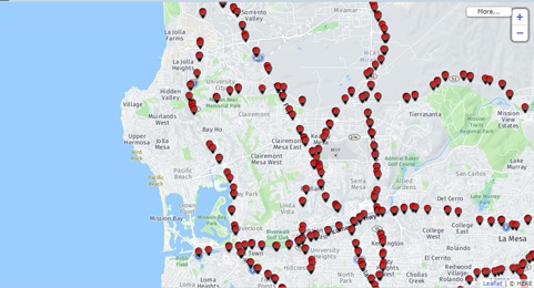
Fig. 1 The traffic detectors distribution in the city of San Diego.
Two detectors are used as the study targets. The location of the two detectors is shown in Fig. 2 and Fig. 3 respectively. The first detector is #1115820 and it is a Main-Lane (ML) type detector that lies on south direction of the Freeway 15. It lies on the edge of the city. It is a medium-level traffic flow detector. The second detector is #1115656 and it is also a Main-Lane (ML) type detector that lies on north direction of the Freeway 15. It lies in a area with high population density. It is a high-level traffic flow detector.
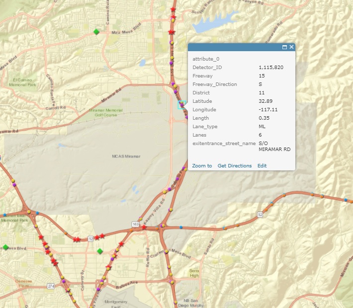
Fig. 2 The traffic detector #1115820.
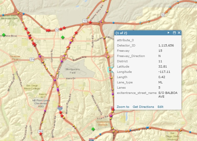
Fig. 3 The traffic detector #1115656.
Traffic flow curves of the two detectors on Jun. 1st, 2017 are shown in Fig. 3 and Fig. 4. It is a Thursday (weekday). We can see the difference between the medium-level and high-level traffic flow detectors.
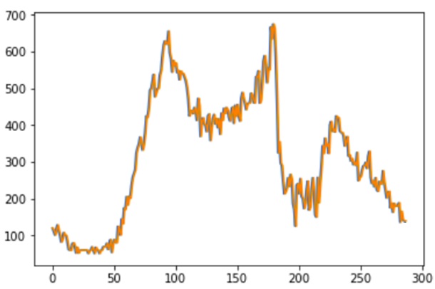
Fig. 4 The traffic flow on Jun. 1st, 2017 of traffic detector #1115820 (sampled every 5min).
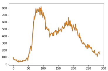
Fig. 5 The traffic flow on Jun. 1st, 2017 of traffic detector #1115656 (sampled every 5min).
The study was conducted with Python3, Jupyter Notebook. The key libraries are pandas, numpy, sklearn, keras, math, matplotlib, os, itertools, sys, datetime and multiprocessing.
List of key python .lib and utilization
| Python .lib | Utilization in Project |
|---|---|
| Pandas | Reading data, Cleaning data, Adding timestamp, Storing data |
| Numpy | Manipulating data, Calculation |
| Datetime | Extracting timestamp information, Measuring training and testing time |
| Sklearn | Scaling data, Training Linear Regression, kNN and SVR model |
| Keras | Building LSTM deep learning prediction model |
| Itertools | Combination of feature sets |
| Multiprocessing | Parallelling programming |
The Advanced Research Computing (ARC) in Virginia Tech is used to realize the big data based study.
The sample of data after data cleaning and formatting is shown in Fig. 6. The first column is 'Time', which stands for the time when the traffic detector record the past 5-minute data. The second column is the 'Detector_ID', which stands for the special ID for each detector. The third column is 'Observed_percent', which stands for the the quality of the detector's measurement. The two detector that are used for this project (#1115820 and #1115656) are both with 100% observed percent. So they are good quality detectors with full observation of the traffic. The forth column is the 'Total_flow', which stands for the aggregated traffic count for the past 5-min. The fifth column is the 'Avg_speed', which stands for the averaged traffic speed during the past 5-min (unit: mph). The sixth column is the number of the data points below 60% observed percent. The seventh column is the number of the data points equal to 100%. The 7th to 13th columns are the timestamps of each data point. The 'Year' is the calendar year. The 'Month' is from 1 to 12. The 'Week' is from 1 to 52. The 'Day' is the day of week and is from 1 to 7. The 'Hour' is the hour of day and is from 1 to 24. The 'Half_Hour' is from 1 to 48. The '15min' is from 1 to 96.
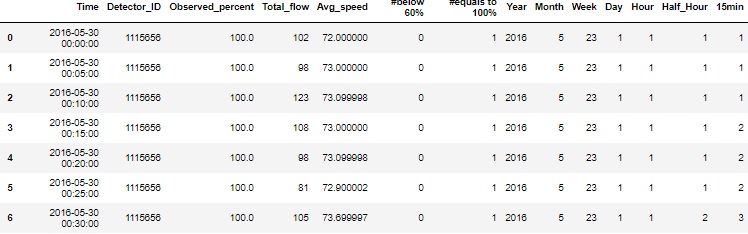
Fig. 6 The data sample of 5-min traffic after data cleaning and formatting.
The data of half-hour traffic is very similar but aggregated every half hour instead of every 5 minutes.
In Fig. 7, in total, 12 features are listed. In general, it can be divided into three classes. First, features 1 to 5 are timestamps. Second, features 6 and 7 are previous one and two traffic data points. Third, features 8 to 12 are averaged historical traffic data points. However, using the whole set of features might cause issue like overfitting and increasing complexity of the training the model. To find the best feature set for predicting the traffic flow, feature sets of 1 to 12 with all possible combination are iterated. The table of feature sets are shown on the right of Fig. 7.
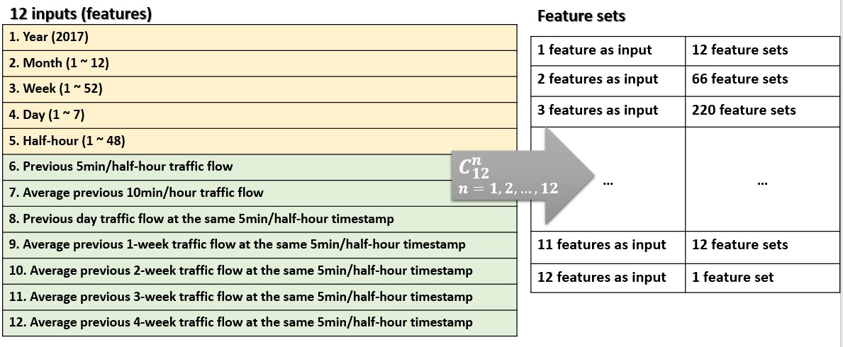
Fig. 7 List of 12 features and n combination (n=1, 2, ..., 12).
In linear regression, the relationships are modeled using linear predictor functions whose unknown model parameters are estimated from the data. Such models are called linear models.(Wikipedia)
The linear regression model is realized with the function from sklearn: linear_model.LinearRegression(normalize=True)
he k-nearest neighbors algorithm (k-NN) is a non-parametric method used for classification and regression. In both cases, the input consists of the k closest training examples in the feature space. The output depends on whether k-NN is used for classification or regression: In k-NN classification, the output is a class membership. An object is classified by a majority vote of its neighbors, with the object being assigned to the class most common among its k nearest neighbors (k is a positive integer, typically small). If k = 1, then the object is simply assigned to the class of that single nearest neighbor. In k-NN regression, the output is the property value for the object. This value is the average of the values of its k nearest neighbors.(Wikipedia)
The kNN model is realized with the function from sklearn: neighbors.KNeighborsRegressor(n_neighbors=n, weights=w, p=p, n_jobs=-1, leaf_size = leaf)
With concern of time limitation, the parameters are fixed instead of iterated to find the best parameter set: n = 7, w = 'distance', p = 1, leaf = 15.
An SVR model is a representation of the examples as points in space, mapped so that the examples of the separate categories are divided by a clear gap that is as wide as possible. New examples are then mapped into that same space and predicted to belong to a category based on which side of the gap they fall. In addition to performing linear classification, SVRs can efficiently perform a non-linear classification using what is called the kernel trick, implicitly mapping their inputs into high-dimensional feature spaces.(Wikipedia)
The SVR model is realized with the function from sklearn: svm.SVR(C=c, epsilon=ep, kernel=k, cache_size=cs)
With concern of time limitation, the parameters are fixed instead of iterated to find the best parameter set: c = 10, ep = 0.001, k = 'rbf', cs = 2000.
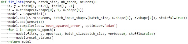
Long short-term memory (LSTM) block or network is a simple recurrent neural network which can be used as a building component or block (of hidden layers) for an eventually bigger recurrent neural network. The LSTM block is itself a recurrent network because it contains recurrent connections similar to connections in a conventional recurrent neural network. An LSTM block is composed of four main components: a cell, an input gate, an output gate and a forget gate. The cell is responsible for "remembering" values over arbitrary time intervals; hence the word "memory" in LSTM. Each of the three gates can be thought of as a "conventional" artificial neuron, as in a multi-layer (or feedforward) neural network: that is, they compute an activation (using an activation function) of a weighted sum. Intuitively, they can be thought as regulators of the flow of values that goes through the connections of the LSTM; hence the denotation "gate". There are connections between these gates and the cell. Some of the connections are recurrent, some of them are not. The expression long short-term refers to the fact that LSTM is a model for the short-term memory which can last for a long period of time. There are different types of LSTMs, which differ among them in the components or connections that they have. An LSTM is well-suited to classify, process and predict time series given time lags of unknown size and duration between important events.(Wikipedia)
With concern of time limitation, the parameters are fixed instead of iterated to find the best parameter set. The key function is defined as below with the functions from keras. The batch_size = 1, nb_epoch = 100, neurons = 4.
To make a fair comparison, 30 days are used for the 5-min traffic flow prediction (8640 data points in total) and 180 days are used for the half-hour traffic flow prediction (8640 data points in total). In this way, the number of data points is kept equal for the two different time-length prediction. The last day is aligned for the two time-length prediction and is used as the testing day (Jun. 1st, 2017, Thur.). The number of the training days is iterated from previous one day (train model on May 31st, 2017, Wed.), previous two days (train model on May 30th and 31st, 2017, Tue. and Wed.), previous three days (train model on May 29th, 30th and 31st, 2017, Mon., Tue. and Wed.), ..., previous 29 / 179 days. Fig. 8 shows the training and testing days alignment and iteration for 5-min and half-hour traffic flow prediction
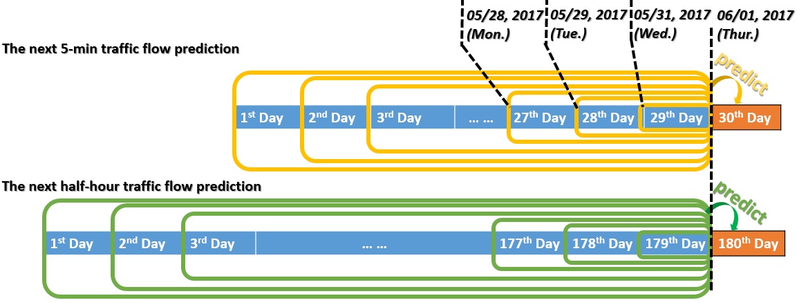
Fig. 8 The training and testing days alignment and iteration for 5-min and half-hour traffic flow prediction.
To evaluate the accuracy of different models, the percentage error SMAPE is used. The SMAPE can be expressed as the equation below:
where y and o represents actual and observed output of test point respectively and N = the number of instances in the test data.
The training and testing time are measured by testing end time minus training start time.
#1115820, next 5-min traffic flow prediction
The SMAPE v.s. the number of features for detector #1115820 is shown in Fig. 9. Because for LSTM, only previous 5-min traffic flow is used as input, Fig. 9 only contains kNN, LR and SVR. For different number of features, the best combination set of features (the smallest SMAPE) is used.
The feature set that produce the lowest SMAPE for Linear Regression is with 8 features (1. Year (2017); 3. Week (1 ~ 52); 4. Day (1 ~ 7); 5. Half-hour (1 ~ 48); 6. Previous 5min traffic flow; 7. Average previous 10min traffic flow; 9. Average previous 1-week traffic flow at the same 5min timestamp; 11. Average previous 3-week traffic flow at the same 5min timestamp) and training on previous 2 days.
The feature set that produce the lowest SMAPE for kNN is with 3 features (6. Previous 5min traffic flow; 7. Average previous 10min traffic flow; 11. Average previous 3-week traffic flow at the same 5min timestamp) and training on previous 1 day.
The feature set that produce the lowest SMAPE for Linear Regression is with 7 features (1. Year (2017); 3. Week (1 ~ 52); 4. Day (1 ~ 7); 6. Previous 5min traffic flow; 8. Previous day traffic flow at the same 5min timestamp; 9. Average previous 1-week traffic flow at the same 5min timestamp; 12. Average previous 4-week traffic flow at the same 5min timestamp) and training on previous 2 days.
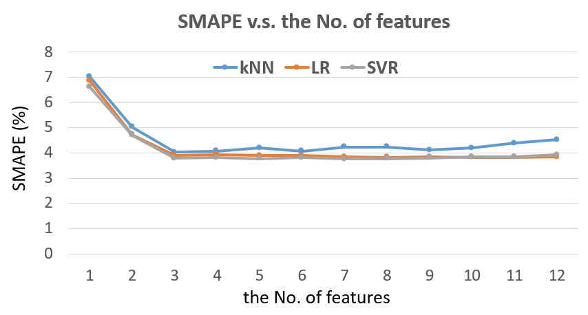
Fig. 9 The SMAPE v.s. the number of features for detector #1115820, next 5-min traffic flow prediction.
From Fig. 9, we can see that increasing the number of features from 1 to 3 brings 3% decrease in SMAPE. However, when increasing to more features than 3 features, the benefit is not so obvious. In application, the number of 3 features is the best choice for input.
Fig. 10 shows the SMAPE v.s. the number of training days for detector #115820. For each number of training days, only the best feature set is used. The Linear Regression shows the lowest SMAPE by training with the previous 2 days and the highest SMAPE by training with the previous 3 days. The kNN shows the lowest SMAPE by training with previous 1 day and the SMAPE starts increase when training with more than 20 days. For kNN, unlike other algorithms show an obvious peak error in training with previous 3 days, it keeps flat within 4 to 4.3% SMAPE before 20 days. The SVR shows quite similar trend as Linear Regression before 20 days but with lower error. Like kNN, SVR also shows increasing SMAPE after 20 days. The LSTM presents the highest error when training with previous less than 20 days. When training with previous more than 20 days, it does not show obvious increase like kNN and SVR, but it is still not better than Linear Regression.
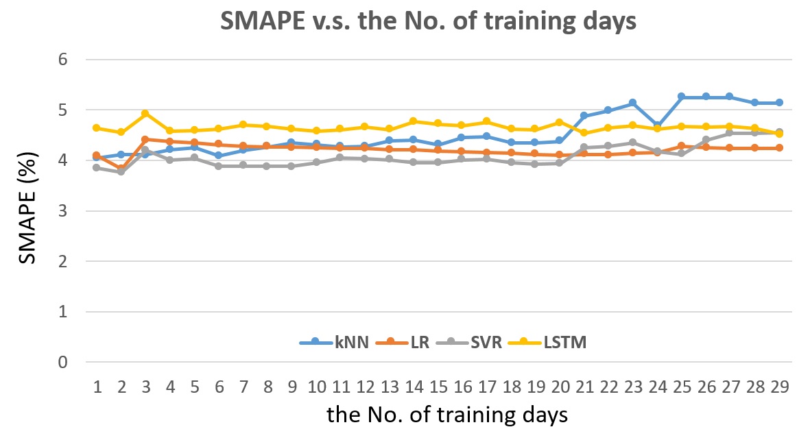
Fig. 10 The SMAPE v.s. the number of training days for detector #1115820, the next 5-min traffic flow prediction.
From Fig. 10, we can see that SVR training within previous 20 days shows the highest accuracy, but we have to be wise on choosing the number of training days. For this case, training on previous 2 days is the best choice while training on 3 days is the worst choice.
Fig. 11 shows the SMAPE v.s. the number of training days with the best feature set. For Linear Regression, it is the 8 features shown in Fig. 9. For the kNN, it is the 3 features shown in Fig. 9. For the SVR, it is the 7 features shown in Fig. 9.
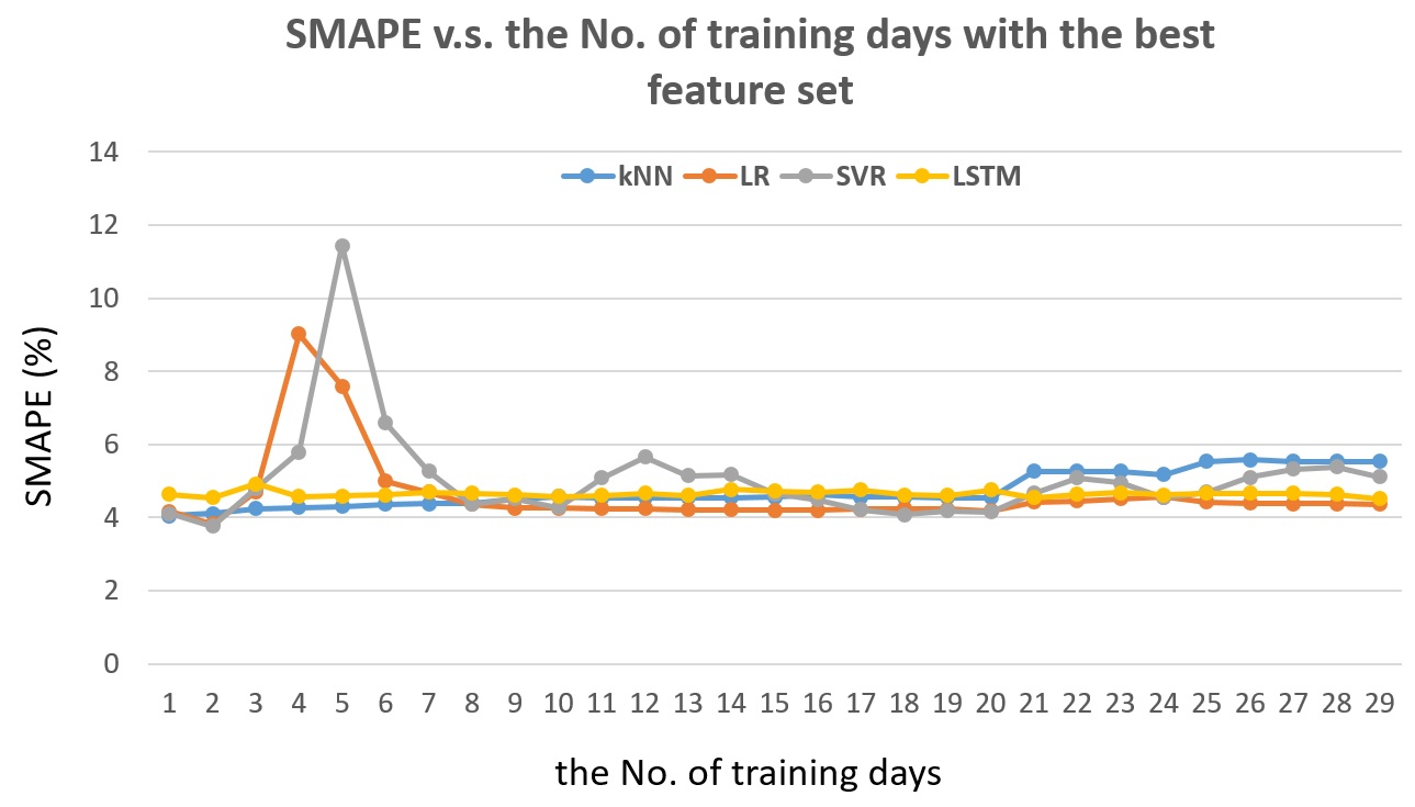
Fig. 11 The SMAPE v.s. the number of training days with the best feature set for detector #1115820, for the next 5-min traffic flow prediction.
From Fig. 11, we can see that by keeping the feature set the same, the training with previous 4 and 5 days brings very high peak error for Linear Regression and SVR. If we check with Fig. 8, we can find that the 4th previous day is Sunday and the 5th previous day is Saturday. The pattern of Sunday and Saturday is very different from the pattern of weekday. For SVR, even training with 2 weeks shows such effect. On the other hand, the kNN and LSTM do not show influence by weekday or weekend. If we compared Fig. 11 with Fig. 10, we can see that by choosing proper set of features, we can actually avoid the severe effect brought by the weekday and weekend difference.
Fig. 12 shows the training and testing time v.s. the number of training days with the best feature set. The y-axis is drawn in log10 portion.
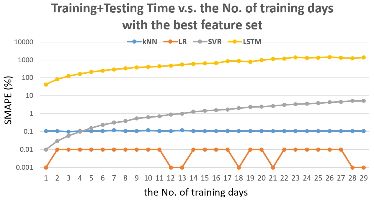
Fig. 12 The training and testing time v.s. the number of training days with the best feature set.
From Fig. 12, we can see that LSTM taks the longest time to train and test and time increases with the increasing of training size. The SVR takes less time than kNN before training within 4 days but increase with the increasing of training size too. The time for Linear Regression and kNN do not increase with increasing of training size. Linear Regression is the fastest one.
From the discussion above and Fig. 9 to 12, SVR should be the best choice that shows the highest accuracy. However, if we take the time into consideration, Linear Regression is the best choice that can be faster and enough accurate.
So, we will use Linear Regression and kNN to study more cases.
#1115820, next half-hour traffic flow prediction
Fig. 13 shows the SMAPE v.s. the number of features for the next half-hour traffic flow prediction. To be efficient, only kNN and Linear Regression are tested. Again, for each number of features, the best set of features training is used. For each number of features, the feature set is different.
For Linear Regression, the best set of features is with 5 features (5. Half-hour (1 ~ 48); 8. Previous day traffic flow at the same half-hour timestamp; 9. Average previous 1-week traffic flow at the same half-hour timestamp; 11. Average previous 3-week traffic flow at the same half-hour timestamp; 12. Average previous 4-week traffic flow at the same half-hour timestamp) and training with 93 days.
For kNN, the best set of features is with 9 features (2. Month (1 ~ 12); 5. Half-hour (1 ~ 48); 6. Previous half-hour traffic flow; 7. Average previous hour traffic flow; 8. Previous day traffic flow at the same half-hour timestamp; 9. Average previous 1-week traffic flow at the same half-hour timestamp; 10. Average previous 2-week traffic flow at the same half-hour timestamp; 11. Average previous 3-week traffic flow at the same half-hour timestamp; 12. Average previous 4-week traffic flow at the same half-hour timestamp) and training with 8 days.
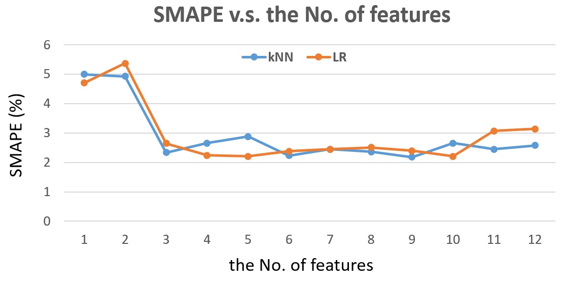
Fig. 13 The SMAPE v.s. the number of features for detector #1115820, next half-hour traffic flow prediction.
From Fig. 13, we can see that the kNN and Linear Regression actually can achieve very similar accuracy. In application, training with 4 features for Linear Regression or training with 3 features for kNN is probably enough to achieve good accuracy.
Fig. 14 shows the SMAPE v.s. the number of training days for the next half-hour traffic flow prediction. For each number of training days, different feature set is chosen to achieve the lowest SMAPE.
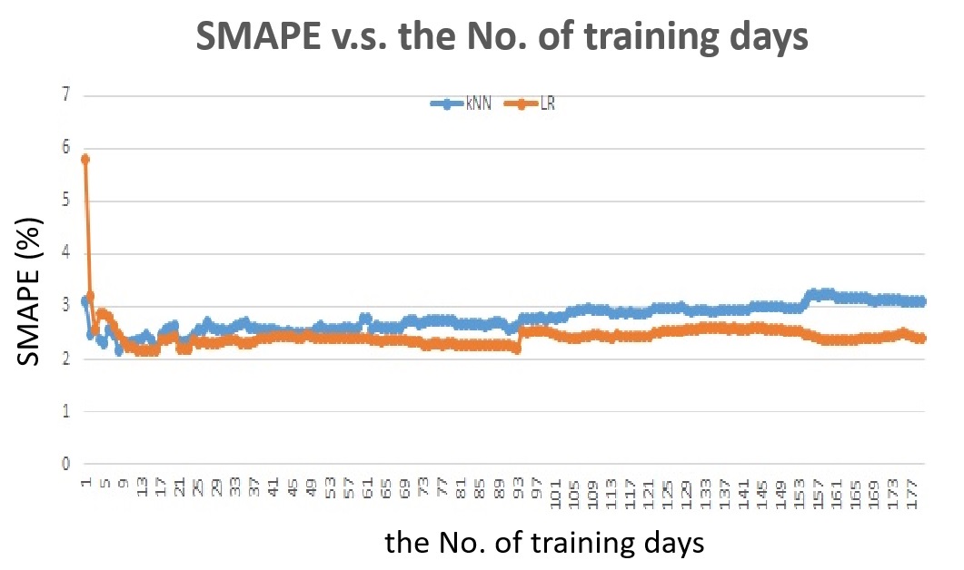
Fig. 14 The SMAPE v.s. the number of training days for detector #1115820, the next half-hour traffic flow prediction.
From Fig. 14, we can see that the Linear Regression does not show good performance wehn training within previous 1 weeks. The SMAPE of the Linear Regression starts to increase after training days increasing to more than 3 months too. So the Linear Regression training is very sensitive the training size and compared with predicting for the next 5-min, the training size should be increased for Linear Regression. On the other hand, the kNN shows good accuracy when training within 2 weeks, it slightly increases with th increasing of training size.
Fig. 15 shows the SMAPE v.s. the number of training days with the best feature set for the next half-hour traffic flow prediction. The feature set is kept the same as the best feature set shown in Fig 13.
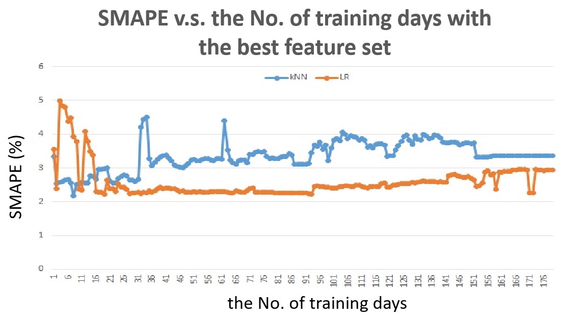
Fig. 15 The SMAPE v.s. the number of training days with the best feature set for detector #1115820, for the next half-hour traffic flow prediction.
Comparing Fig. 14 with Fig. 15, we can see that the feature set for kNN actually varies a lot when changing the training size to achieve good accuracy. Linear Regression does not show good performance for training size within 2 weeks but the performance is very good when training size is from 2 weeks to 3 months.
From the discussion above and Fig. 13 to 15, predicting the next half-hour traffic flow requires more training days than the prediction of the next 5-min to achieve good accuracy. As in real application, the feature set will probably be fixed, the Linear Regression that shows stable performance with only one feature set is preferred rather than kNN.
#1115656, next 5-min traffic flow prediction
Fig. 16 shows the SMAPE v.s. the number of features for the next 5-min traffic flow prediction. For each number of features, different feature sets are compared to find the best feature set with the number.
For Linear Regression, the best feature set is achieved by 5 features (1. Year (2017); 3. Week (1 ~ 52); 6. Previous 5min traffic flow; 7. Average previous 10min traffic flow; 10. Average previous 2-week traffic flow at the same 5min timestamp) and training with previous 2 days.
For kNN, the best feature set is achieved by 6 features (2. Month (1 ~ 12); 5. Half-hour (1 ~ 48); 6. Previous 5min traffic flow; 7. Average previous 10min/hour traffic flow; 10. Average previous 2-week traffic flow at the same 5min timestamp; 11. Average previous 3-week traffic flow at the same 5min timestamp) and training with previous 4 days.
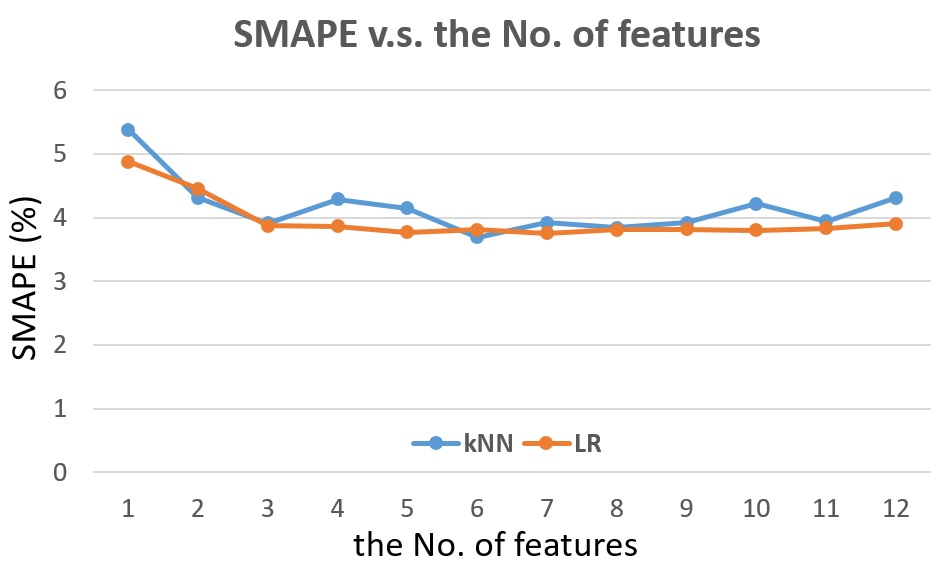
Fig. 16 The SMAPE v.s. the number of features for detector #1115656, next 5-min traffic flow prediction.
From Fig. 16, we can see that while kNN shows the lowest error, it shows the sensitivity to different number of feature set. For Linar Regression, when feature set reaches the number of 5, the accuracy is kept quite stable.
Fig. 17 shows the SMAPE v.s. the number of training days for the next 5-min traffic flow prediction. For each number of training days, different feature sets are compared to find the best feature set for that number of training days.
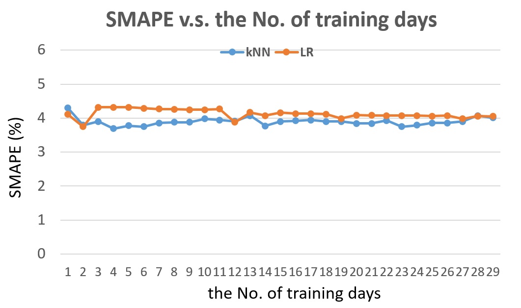
Fig. 17 The SMAPE v.s. the number of training days for detector #1115656, the next 5-min traffic flow prediction.
From Fig. 17, we can see that for kNN, by choosing different feature set, the accuracy of its prediction is always better than the accuracy of Linear Regression.
Fig. 18 compares the Linear Regression and the kNN with the same feature set. Similar to the previous observation, kNN is quite insensitive the weekday and weekend. The performance of kNN with the best feature set shown above is quite good and stable to the training size.

Fig. 18 The SMAPE v.s. the number of training days with the best feature set for detector #1115656, for the next 5-min traffic flow prediction.
From Fig. 18, we can see that for detector #11115656, kNN performs better than Linear Regression with better accuracy and insensitivity to training dataset.
#1115656, next half-hour traffic flow prediction
Fig. 19 shows the SMAPE v.s. the number of features for detector #1115656 for the next half hour traffic flow prediction.
For Linear Regression, the best prediction is achieved by training with 6 features (2. Month (1 ~ 12); 3. Week (1 ~ 52); 7. Average previous hour traffic flow; 8. Previous day traffic flow at the same half-hour timestamp; 10. Average previous 2-week traffic flow at the same half-hour timestamp; 12. Average previous 4-week traffic flow at the same half-hour timestamp) and trainign for the previous 1 day.
For kNN, the best prediction is achieved by training with 6 features (1. Year (2017); 5. Half-hour (1 ~ 48); 7. Average previous hour traffic flow; 9. Average previous 1-week traffic flow at the same half-hour timestamp; 10. Average previous 2-week traffic flow at the same half-hour timestamp; 11. Average previous 3-week traffic flow at the same half-hour timestamp) and training for the previous 20 days.
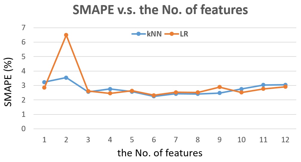
Fig. 19 The SMAPE v.s. the number of features for detector #1115656, next half-hour traffic flow prediction.
From Fig. 19, we can see that both kNN and Linear Regression achieve best performance with 6 features. The kNN is a little bit better than the Linear Regression.
Fig. 20 shows the SMAPE v.s. the number of training days for the next half-hour traffic prediction. While Linear Regression shows good performance when training with 3 days, the error sharply increases when training with previous number of days between 3 to 40. kNN shows much stable performance and achieves the best performance when training with previous 20 days.
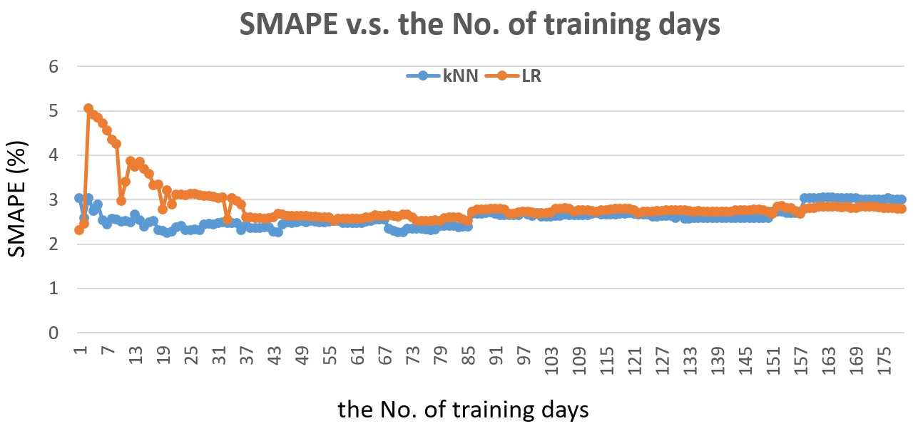
Fig. 20 The SMAPE v.s. the number of training days for detector #1115656, the next half-hour traffic flow prediction.
Fig. 21 show the SMAPE v.s. the number of training days with the best feature set for the next half-hour traffic flow prediction. The performance of kNN is more stable and better than that of Linear Regression when training within the previous 150 days. The sharp increase of kNN prediction error at the day 156 needs further study to explain.
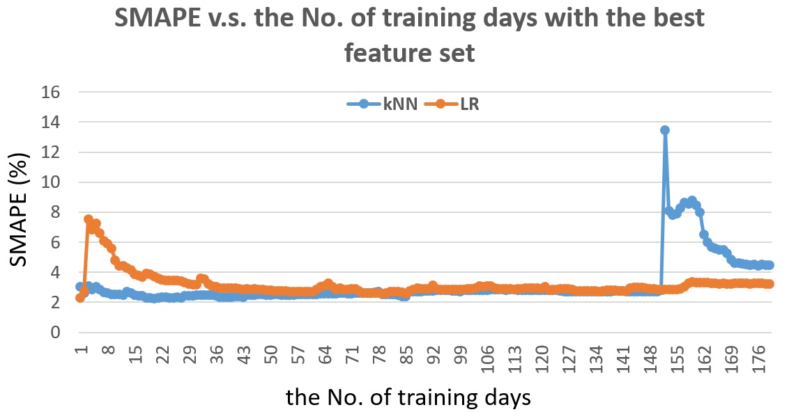
Fig. 21 The SMAPE v.s. the number of training days with the best feature set for detector #1115656, for the next half-hour traffic flow prediction.
In this project. Four machine learning algorithms are used in traffic prediction application. Linear Regression is the fastest and fairly good one. SVR can build the most accurate prediction model but the training time increases with the training size. kNN is a non-parametric algorithm and shows comparable performance to Linear Regression. LSTM is one deep learning algorithm and also shows stable performance.
With the results shown in the previous session, we can conlude that:
- For a medium traffic flow detector (#1115802), Linear Regression shows the best performance when taking both the accuracy and the training time into consideration. In application, training with 3 to 4 features is enough to achieve good accuracy for both the next 5-min and half-hour prediction.
- For a high traffic flwo detector (#1115656), kNN shows the best performance. In application, training with 5 to 6 features is enough to achieve good accuracy for both ethe next 5-min and half-hour prediction.
- When using Linear Regression and SVR, weekend needs to be avoided while kNN and LSTM do not have such issue.
- For the training size, when predicting the next 5-min, training within 1 week shows the best performance. When predicting the next half-hour, training around 20 days shows the best performance.
One issue of the work is that the parameters of the kNN, SVR and LSTM is pre-defined instead of iteration over ranges to find the best set of parameters to save time. If the validation procedure is applied, the performance of SVR, kNN and LSTM might be improved but it will takes much longer time to get the results.
[1] Gregory J. Grindey, S. Massoud Amin, Ervin Y. Rodin, Asdrubal Garcia-Ortiz, "Kalman filter approach to traffic modeling and prediction," Intelligent Transportation Systems (ITS), doi: 10.1117/12.300860, 1998.
[2] C. Moorthy and B. Ratcliffe, “Short term traffic forecasting using time series methods,” Transp. Plan. Technol., vol. 12, no. 1, pp. 45–56, Jul. 1988.
[3] H. J. H. Ji, A. Xu, etc., “The applied research of Kalman in the dynamic travel time prediction,” in Proc.18th Int. Conf. Geoinformat., 2010, pp. 1–5.
[4] B. Pan, U. Demiryurek, and C. Shahabi, “Utilizing real-world transportation data for accurate traffic prediction,” in 2012 IEEE 12th International Conference on Data Mining (ICDM). IEEE, 2012, pp. 595–604.
[5] B. Pan, U. Demiryurek, and C. Shahabi. “Utilizing real-world transportation data for accurate traffic prediction,” IEEE 12th International Conference on Data Mining (ICDM), pp 595-604, Dec 2012.
[6] Lippi M, Bertini M, Frasconi P. Short-term traffic flow forecasting: an experimental comparison of time-series analysis and supervised learning. IEEE Transactions on Intelligent Transportation Systems 2013; 14(2): 871–882.
[7] G. A. Davis and N. L. Nihan, “Nonparametric regression and short-term freeway traffic forecasting,” J. Transp. Eng., vol. 117, no. 2, pp. 178–188,Mar./Apr. 1991.
[8] J. Wang, Q. Gu, J. Wu, etc., Traffic Speed Prediction and Congestion Source Exploration: A Deep Learning Method 2016, IEEE 16th International Conference on Data Mining.
[9] Y. Lv, Y. Duan, W. Kang, Z. Li, and F.-Y. Wang, “Traffic flow prediction with big data: A deep learning approach,” Intelligent Transportation Systems, IEEE Transactions on, vol. 16, no. 2, pp. 865–873, 2015.
[10] Long short-term memory neural network for traffic speed prediction using remote microwave sensor data, Transportation Research Part C, 2015.
[11] J. Zhu and T. Zhang, “A layered neural network competitive algorithm for short-term traffic forecasting,” in Proc. CORD Conf., Dec. 2009, pp. 1–4.
[12] E.Y. Kim, MRF model based real-time traffic flow prediction with support vector regression, IET 2017 Feb.
[13] M. T. Asif, J. Dauwels, C. Y. Goh, A. Oran, E. Fathi, M. Xu, M. M. Dhanya, N. Mitrovic, and P. Jaillet, “Spatiotemporal patterns in large-scale traffic speed prediction,” Intelligent Transportation Systems, IEEE Transactions on, vol. 15, no. 2, pp. 794–804, 2014.