Gaussian Belief Propagation for MIMO detector
Wei ChenSpring 2014 ECE 6504 Probabilistic Graphical Models: Class Project
Virginia Tech
Goal
This project intends to study the MIMO decoding with PGM method. MIMO technologies are broadly used in wireless communication system, like 3G/4G/WiFi standards. As most modern wireless communication technologies have been reaching Shannon limit, MIMO technology are used as one of major technologies to increase whole system capacity. Future technology may use much larger MIMO arrays to get higher throughput/lower transmit power/better coverage. The MIMO detector performance and implementation cost are hence critical for real system design. There are three major type of MIMO detectors which were studied in recent years, sphere decoding, channel truncation and graph based detection. In this project GPM based detector MiMo detector is studied.1 Introduction
Multiple Input Multiple Output(MIMO) system are widely used in wireless technologies. MIMO systems have shown their capability to significantly improve both channel capacity and error rate performance. For an example, current deployed LTE system has 2 8 antennas at base station side, which can provide up to 300Mbps peak throughput (LTE). Very large MIMO system can offer very high spectral efficiencies.
The optimal way for MIMO detector is to use a maximum a posteriori (MAP) or maximum likelihood(ML) detector. However the computational complexity increases exponentially with the number of antennas. MAP detector has complexity as O(LN). Spatial filtering(MMSE, ZF) has complexity as O(N3). For a MIMO system with 100+ antennas, the computational complexity with these methods are prohibitive. So recently methods with probabilistic graphics model were studied as a competitive solution for MIMO detector. We will discuss later, although running belief propagation on a fully connected Markov Random Field (MRF) has same complexity as MMSE detector, there are many proposals to reduce the complexity of BP detector, some detectors can have complexity as O(N2)
2 System and Channel Model
2.1 System description
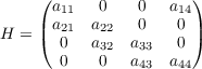
For a MIMO system with NT transmit and NR receive antennas, can be modeled as
 | (1) |
From transmitter side, information were modulated and mapped on to all NT antennas. The narrowband
channel is represented by a matrix H of size NR ×NT, where each entry hi,j defines a channel connecting
transmit antenna j and receive antenna i. The received signal, Y is the received vector of length NR, and
noise N is a vector of Gaussian noise: N ~ (0,σn2I)

2.2 Optimal detection
The optimal MAP detector enumerates all the elements of the joint posterior distribution
 | (2) |
and then marginalizes out each variables:
 | (3) |
Since we assume that the noise vectors, a jointly Gaussian complex random variables, are also i.i.d and with with zero mean and same variance σn2, then the pdf of noise vector can be shown as
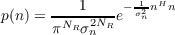 | (4) |
Assume that H is known for receiver by other means(Channel Estimation). Since n = y - Hx, we get
 | (5) |
For most likelihood estimator, maximize equation 2 is not maximize equation 5. Maximize equation 5 is same to
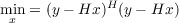 | (6) |
Expand equation 6 and from the derivative, we can conclude that the optimal solution is
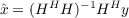 | (7) |
Here the MAP detector is same as MMSE detector since the model and mean of gaussian distribution are same. MMSE detection has complexity of O(N3), it becomes intractable even for configurations of moderate size.
2.3 Using belief propagation
In order to reduce the complexity of decoder, approximate algorithms were proposed. We can expand equation 2 and equation 5 to get the P(x∣y,H). The joint distribution can be expressed as
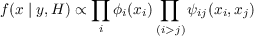 | (8) |
where
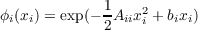
![ϕi(xi) = exp[xizi + log p(xi)]](6504_MiMo20x.png) | (9) |
 | (10) |
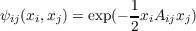
 | (11) |
 | (12) |
The values of ϕi(xi) and ψi,j(xi,xj) given by equation 9 and equation 11 can be treated as node potentials
and edge potentials of an undirected graphical model to which we can apply belief propagation.
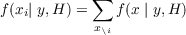
Belief propagation tries to estimate the marginal probabilities for all variables by means of passing messages between local nodes. The local belief at every node is calculated as the product of the local evidence and all incoming messages
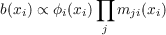 | (13) |
where the message from node j to i, mji(xi) represents the state in which xi should be according to node j.
From equation 7 we can also get similar presentation. As presented in [5], equation 7 can be rewritten as a linear problem form Ax = b,
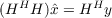 | (14) |
where A = (HHH) and b = HHy. Linear problem can be solved with Gaussian Belief Propagation. The idea is to convert Ax = b to an optimization problem
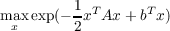 | (15) |
while define a PDF as p(x) =  -1exp(-
 xTAx + bTx). This is PDF is a multivariate gaussian distribution
with (A-1b,A-1). Since A = (HHH) and b = HHy, the PDF is now ((HHH)-1b,(HHH)-1).
This PDF can be rewritten similar with equation 8 while
xTAx + bTx). This is PDF is a multivariate gaussian distribution
with (A-1b,A-1). Since A = (HHH) and b = HHy, the PDF is now ((HHH)-1b,(HHH)-1).
This PDF can be rewritten similar with equation 8 while
 | (16) |
 | (17) |
Comparing equations from 8 to 12 with equation 16 17, we can see if we assume that P(xi) is a constant,
which is true for scrambled encoder, two solutions are almost same with similiar node/edge potentials on a
pairwise MRF.
As deducted above, MIMO detector can use Gaussian belief propagation as a iterative solution. But unfortunately, although the channel matrix H could be sparse, HHH is a matrix with high density, so the complexity is still high when the matrix size is big.
3 Gaussian belief propagation Algorithms
3.1 means and variance
Gaussian Belief Propagation(GaBP) is a special case of continues belief propagation. Since the
underlying distribution is Gaussian, the algorithms can be simplified with simply rules, message
propagated are means and variance of distribution. There are some basic properties of gaussian
distribution which could be used to simplify message passing. As derived in [5], if there are two
gaussian random variables density functions (μ1,P1-1),(μ2,P2-1), the product of two
functions is also a gaussian distribution with (μ,P-1), where μ = P-1(P1μ1 + P2μ2) and
P-1 = (P1 + P2)-1
There is another interesting properties of gaussian belief propagation. Since gaussian distribution mode and mean are same, the max-product version of belief propagation and sum-product version of belief propagation are identical[5]. Since all messages are gaussian variables. Messages between different nodes can be simplified as message of mean and variance of a gaussian distribution.
 | (18) |
Details of GaBP algorithms and matlab code can be found in [5].
3.2 correctness of convergence
Another interesting property of Gaussian belief propagation is the correctness of convergence. As studies of Turbo code and other topics demonstrated, Gaussian belief propagation converges to right means even with loopy topology. Weiss and Freeman [9] proved that with concept of ”unwrapped tree”, GaBP converges to right posterior means on any arbitrary topology, with single loop and with many loops.
4 Simplified graph model for MiMo
4.1 graphical model on channel matrix
In section 2.3, we conclude that GaBP can executed on a MRF represented by matrix HHH. To get this
matrix, a matrix multiplication need to be performed, also the result matrix is a dense matrix, the
complexity is still too high.
D.Bickson proposed to construct an alternative matrix  In[5].
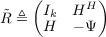 | (19) |
where Ψ = σ2I is the AWGN diagonal noise. And then define new vector of variables  ≜{
≜{ T,zT}T,
where
T,zT}T,
where  is the soution vector and z is an auxiliary vector. The new observation vector is
  ≜{0T,yT}T.
Then
≜{0T,yT}T.
Then
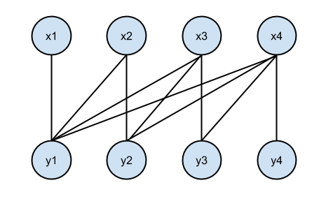
 | (20) |
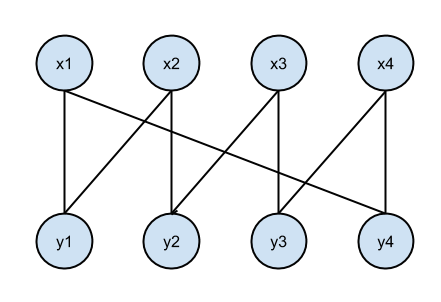
This equation is similar with the graph proposed by Montanari in [2] for CDMA multi-user detection. The graph model is exact what is shown in 1, a bipartite graph with Nt node at one side and Nr nodes at other side. Although Montanari’s graph model is DAG, the graph model derived from equation 19 and equation 20 is a UAG, which provides additional convergence and simpler update rules.
4.2 further simplified graphic models
The graphical model used in last section still a full connected graph with Nt × Nr edges. To reduce the
computational burden of message passing and marginalization, different solutions were studied. In[7]
Hu&Duman proposed to prune some edges for thick the corresponding variable and observation nodes are
weakly coupled together. The problem with this method is that we can not prune too many edges to ensure
reasonable performance.
An alternative strategy to prune edges is to prune edges via linear transformation. As mentioned in
introduction, sphere decoding is an algorithms widely used to decode MiMo. In sphere decoding, the QR
decomposition is first used to trianglularize the channel and then a tree search is applied for post joint
detection. In QR decomposition, the channel matrix H is decomposed into H = QR, here Q is square
matrix that QHQ = I and R is an upper triangular matrix. Then the original problem is projected to new
coordination y′ = QHy = Rx + QHn. If we run GaBP for this problem, the graphic model is shown in Fig
2. The total edges in GPM are 10 for a 4 × 4 MiMo system, 6 edges less than a full connected graph.
Another transformation studied [8] is bi-diagonalization of channel matrix, or it is called channel truncation, where the effective channel is given by
 | (21) |
In [8], Viterbi algorithm was proposed to solve this formation, in PGM, it also has a straightforward model. With this channel matrix the GPM for a 4 × 4 MiMo channel can be shown as in Fig 3(a). Fig 3(b) is a re-arrangement Fig 3(a), which is basically a ring type of PGM. Total edges for a 4 × 4 MiMo system is 8. In[1], the ring type PGM MiMo detector was evaluated and the performance was reasonable after 4 6 iterations, with 0.3~1.0 dB difference.
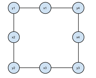
Also as shown in [10], GaBP can be implemented with Gilbert Multiplier circuit directly. They demonstrated a MIMO detector with this analog circuit for the loopy structure shown in Fig 3(b), which provides a possibility to implement MIMO signal processing tasks with low-power analog circuity in continues time domain.
5 Conclusion
In the project, GPM based MiMo detector was studied, GPM built upon the original channel matrix was studied, further channel truncation and sphere MiMo detectors equivalent GPM model was introduced. With the proven algorithms as channel truncation and sphere detector, GPM version provides an iterative method with less computation burden. As suggested in other works, the GPM solution have more advantages for large MiMo system ISI channel, where the 3D channel matrix is big and sparse.
6 Reference
[1] Seokhyun Yoon, Jun Heo. Pair-wise Markov Random Fields Applied to the Design of Low Complexity MIMO detectors.
[2] Andrea Montanari, Balaji Prabhakar, David Tse. Belief Propagation Based Multi-User Dection.
[3] D.Bickson, O.Shental, PH.Siegel, J.K.Wolf, D.Dolev. Gaussian belief propagation based multiuser detection.
[4] J Soler-Garrido, R.J.Picchocki, K. Maharatna, D.McNamara. Analog MIMO detection on the basis of belief propagation
[5] Danny Bickson, Gaussian Belief Propagation:Theory and Application
[6] A Montanari, B Prabhakar, D Tse, Belief Propagation Based Multi-user detection
[7] Jun.Hu, T.M.Duman, Graph based detector for BLAST architecture
[8] Wen.Jiang,Ye,Li, XingXing Yu, 2007. Truncation for Low-Complexity MIMO signal detection.
[9] Y.Weiss ,W.T.Freeman, 1999, Correctness of belief propagation in Gaussian Graphical models of arbitrary Topology”
[10] J.S.Garrido, R.J.Picchocki, K.Maharatna 2006, Analog MIMO detection on the basis of belief propagation.